Time-domain Granger Causality

Pairwise Granger Causality

The Granger causality is a method to determine functional connectivity between time-series using autoregressive modelling. In the simpliest pairwise Granger causality case for signals X and Y the data are modelled as autoregressive processes. Each of these processes has two representations. The first representation contains the history of the signal X itself and a prediction error (or noise a.k.a. residual), whereas the second also incorporates the history of the other signal.

If inclusion of the history of Y next to the history of X into X model reduces the prediction error compared to just the history of X alone, Y is said to Granger cause X. The same can be done by interchanging the signals to determine if X Granger causes Y.

Conditional Granger Causality

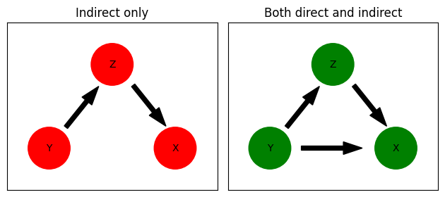
Conditional Granger causality can be used to further investigate this functional connectivity. Given signals X, Y and Z, we find that Y Granger causes X, but we want to test if this causality is mediated through Z. We can use Z as a condition for the aforementioned Granger causality.

In order to illustrate the function of time-domain Granger causality we will be using examples from Ding et al. (2006) chapter. Specifically, we will have two cases of three signals. In the first case we will have indirect connectivity only, whereas in the second case both direct and indirect connectivities will be present.

References: Ding M., Chen Y. and Bressler S.L. (2006) Granger Causality: Basic Theory and Application to Neuroscience. https://arxiv.org/abs/q-bio/0608035

import matplotlib.pyplot as plt
import numpy as np
from elephant.causality.granger import pairwise_granger, conditional_granger
from elephant.datasets import load_data

fig, (ax1, ax2) = plt.subplots(nrows=1, ncols=2)
# Indirect causal influence diagram
node1 = plt.Circle((0.2, 0.2), 0.1, color='red')
node2 = plt.Circle((0.5, 0.6), 0.1, color='red')
node3 = plt.Circle((0.8, 0.2), 0.1, color='red')
ax1.set_aspect(1)
ax1.arrow(0.28, 0.3, 0.1, 0.125, width=0.02, color='k')
ax1.arrow(0.6, 0.5, 0.1, -0.125, width=0.02, color='k')
ax1.add_artist(node1)
ax1.add_artist(node2)
ax1.add_artist(node3)
ax1.text(0.2, 0.2, 'Y', horizontalalignment='center', verticalalignment='center')
ax1.text(0.5, 0.6, 'Z', horizontalalignment='center', verticalalignment='center')
ax1.text(0.8, 0.2, 'X', horizontalalignment='center', verticalalignment='center')
ax1.set_title('Indirect only')
ax1.set_xbound((0, 1))
ax1.set_ybound((0, 0.8))

ax1.tick_params(axis='both', which='both', bottom=False, top=False, labelbottom=False,
                right=False, left=False, labelleft=False)

# Both direct and indirect causal influence diagram
node1 = plt.Circle((0.2, 0.2), 0.1, color='g')
node2 = plt.Circle((0.5, 0.6), 0.1, color='g')
node3 = plt.Circle((0.8, 0.2), 0.1, color='g')
ax2.set_aspect(1)
ax2.arrow(0.28, 0.3, 0.1, 0.125, width=0.02, color='k')
ax2.arrow(0.35, 0.2, 0.2, 0.0, width=0.02, color='k')
ax2.arrow(0.6, 0.5, 0.1, -0.125, width=0.02, color='k')
ax2.add_artist(node1)
ax2.add_artist(node2)
ax2.add_artist(node3)
ax2.text(0.2, 0.2, 'Y', horizontalalignment='center', verticalalignment='center')
ax2.text(0.5, 0.6, 'Z', horizontalalignment='center', verticalalignment='center')
ax2.text(0.8, 0.2, 'X', horizontalalignment='center', verticalalignment='center')
ax2.set_xbound((0, 1))
ax2.set_ybound((0, 0.8))

ax2.tick_params(axis='both', which='both', bottom=False, top=False, labelbottom=False,
                right=False, left=False, labelleft=False)
ax2.set_title('Both direct and indirect')
plt.tight_layout()
plt.show()

Indirect causality

First we load three time series with indirect connectivity only, i.e., there is a functional connectivity from time series Y to X mediated solely through a third time series Z.

The time series are automatically generated and stored into a neo.AnalogSignal object, where the first dimension defines the time samples, and the second dimension each series. The time series are ordered X, Y, Z, and acessible with indexes 0, 1, and 2, respectively.

np.random.seed(1)

# Indirect causality
xyz_indirect_sig = load_data('granger_causality_indirect')
xy_indirect_sig = xyz_indirect_sig[:, :2]
indirect_pairwise_gc = pairwise_granger(xy_indirect_sig, max_order=10, information_criterion='aic')
print(indirect_pairwise_gc)

Causality(directional_causality_x_y=0.0, directional_causality_y_x=0.4, instantaneous_causality=0.0, total_interdependence=0.4)

/home/docs/checkouts/readthedocs.org/user_builds/elephant-docs-development/conda/latest/lib/python3.12/site-packages/elephant/causality/granger.py:677: UserWarning: The value of the log determinant is at or below the tolerance level. Proceeding with computation.
  warnings.warn("The value of the log determinant is at or below the "

# Indirect causality (conditioned on z)
indirect_cond_gc = conditional_granger(xyz_indirect_sig, max_order=10, information_criterion='aic')
print(indirect_cond_gc)
print('Zero value indicates total dependence on signal Z')

0.0
Zero value indicates total dependence on signal Z

Both direct and indirect causality

Now we load three time series with both direct and indirect connectivity. Therefore, there is functional connectivity from the time series Y to X mediated by direct connections from Y to X and indirect connections mediated by the third time series Z.

# Both direct and indirect causality
xyz_both_sig = load_data('granger_causality_both')
xy_both_sig = xyz_both_sig[:, :2]
both_pairwise_gc = pairwise_granger(xy_both_sig, max_order=10, information_criterion='aic')
print(both_pairwise_gc)

Causality(directional_causality_x_y=0.0, directional_causality_y_x=0.73, instantaneous_causality=0.0, total_interdependence=0.73)

# Both direct and indirect causality (conditioned on z)
both_cond_gc = conditional_granger(xyz_both_sig, max_order=10, information_criterion='aic')
print(both_cond_gc)
print('Non-zero value indicates the presence of direct Y to X influence')

0.08
Non-zero value indicates the presence of direct Y to X influence